

V4r3 User Guide
Documentation Files
| Name | Description |
|---|---|
| README | File containing information |
| V4r3_estimation_synopsis.pdf | Synopsis of V4r3 estimation |
| V4r3_output_fields.pdf | Overview of V4r3 files |
| V4r3_overview_plots.pdf | Plots of V4r3 |
| V4r3_input_data.pdf | Data used in V4r3 |
| evaluating_budgets_in_eccov4r3_updated_20220118.pdf | Calculating budgets with V4r3 output |
| V4r3_reproduction_howto.pdf | Reproducing V4r3 results with MITgcm |
| available_diagnostics.log | A full list of available diagnostics with a short description (for a slightly more detailed description of diagnostics, check out the readme file*) |
| costfunction0059 | Costs with the grid size factor (gamma, Cf. V4r3_summary.pdf for an explanation of gamma) |
| costfunction0059_nogamma | Costs without the grid size factor (gamma) |
| STDOUT.0000 | Model standard output |
1. Introduction
This note describes the directory structure and content of ECCO Version 4, Release 3's (V4r3) repository. Covering the time period from 1992 through 2015, ECCO V4r3 synthesizes a general circulation model (MITgcm) and most of available satellite and in situ data to produce a physically consistent ocean estimate of which property budgets can be closed. The data that are used to constrain the model include satellite altimetry (sea surface height, SSH), GRACE ocean bottom pressure (OBP), AVHRR sea surface temperature (SST), Aquarius sea surface salinity (SSS), Argo, CTD, XBT, mooring temperature and salinity data, sea-ice measurements, and global mean SSH and OBP. The estimate uses the adjoint method to iteratively minimize a cost function that is defined as the sum of the squared sum of weighted model-data misfits and control adjustments. ECCO V4r3 is the final product after a series of iterations. A detailed summary of the estimate can be found in Fukumori et al. (2017).
2. Model
The model that is used to produce V4r3 is MITgcm version checkpoint66g. Wang et al. (2017) gives a detailed description about how to download the code, data, and any needed auxiliary files to reproduce V4r3.
The grid used in V4r3 is the so-called LLC90 (Lat-Lon-Cap 90) grid (Fig. 1a) that has five faces covering the whole globe, with simple latitude-longitude grid between 70°S and 57°N and an Arctic cap (Forget et al., 2015). The dimensions for the five faces are [90x270], [90x270], [90x90], [270x90], and [270x90] where each face consists of tiles dimensioned 90x90 (thus LLC90) (Figs. 1a & 1b). The horizontal resolution varies spatially from 22km to 110m, with the highest resolution in high latitudes and lowest resolution in mid latitudes. The deepest ocean bottom is set to 6145m below the surface, with the vertical grid spacing increasing from 10m near the surface to 457m near the ocean bottom.
3. Directory Structure
In this section, we describe the directory structure of V4r3's repository. Each subdirectory has a short README file that lists all the sub-directories and files in that directory along with a brief description. The directory structure is similar to that of Release 2's (Forget et al., 2016).
3.1 Documentation
The directory doc contains a few useful documents that include an overview of the repository, a summary of V4r3 (Fukumori et al., 2017), a note about how to reproduce V4r3 results (Wang, 2018), a set of analysis plots generated using gcmfaces (see Software below), and a note on analyzing budgets (Piecuch, 2022). Also included are summary files of all cost functions (costfunction*) and a "standard output file" (STDOUT.0000) that the model creates during its integration with useful information about the model configuration and measures of the model state.
3.2 Model Grid

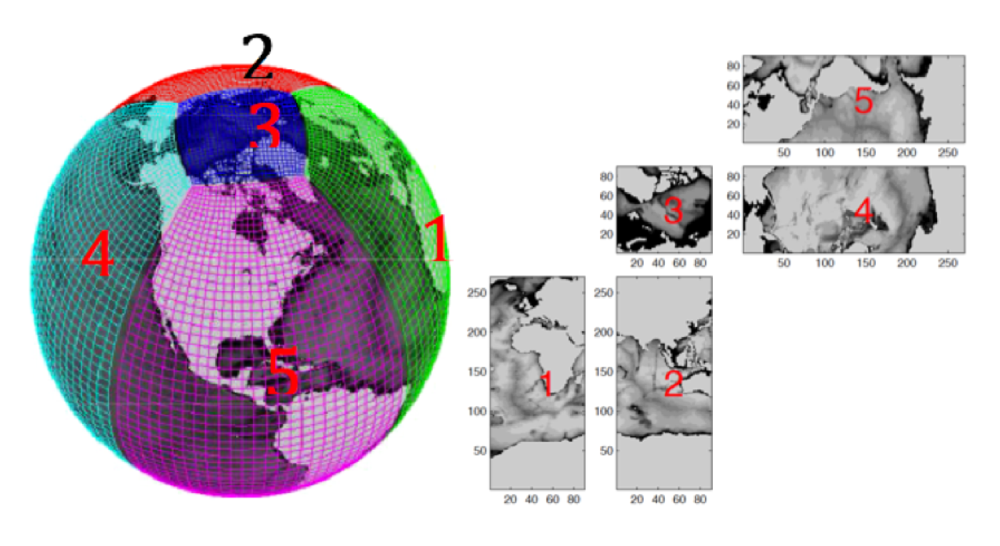
The model grid information can be found in the subdirectory nctiles_grid. The globe is split into 13 regional tiles (Fig. 2, courtesy of Gaël Forget), with variables of which are saved in separate individual files in netCDF format. In Section 5 (Software), we provide an example MATLAB script to read in the model grid by making use of gcmfaces, a MATLAB toolbox developed by Gaël Forget from Massachusetts Institute of Technology (MIT) (Forget, 2017).
3.3 Monthly Average Model Fields
The nominal model output is its monthly fields (nctiles_monthly). Each subdirectory inside nctiles_monthly contains netCDF files for a particular variable, as indicated by the name of the subdirectory, split into 13 files as described above. Some of the most commonly used fields, like velocity components, potential temperature, salinity, SSH, and OBP are UVEL, VVEL, THETA, SALT, SSH, and OBP, respectively. An example of MATLAB script is provided in Section 5 (Software) to read and display these netCDF files (Box 2).
3.3.1 Corrected Sea Level and Ocean Bottom Pressure
There are two variables, ETAN and SSH, describing sea surface height. ETAN is the height of the model's liquid ocean surface, whereas SSH is the dynamic sea surface height plus global mean steric sea level change. ETAN is located below sea-ice where it exists, due to pressure loading from the ice and snow on top. SSH corrects ETAN for this loading (dynamic sea surface height) and further adds a correction for the global mean steric height change, the so-called Greatbatch correction (Griffies and Greatbatch, 2012). Both variables reflect mass changes caused by freshwater input. As such, variable SSH provides the model equivalent of altimetry sea level measurements.
Similarly, there are two variables, PHIBOT and OBP, for ocean bottom pressure. PHIBOT represents the model's ocean bottom pressure (including sea-ice loading), while OBP corrects PHIBOT for global mean steric height change. Variable OBP provides the model equivalent of GRACE OBP.
3.3.2 Native and Geographical Velocity Components
Users are advised to be aware of the directional convention used in the model especially when analyzing the vector fields of the model. Figure 1b illustrates the directional convention used in the LLC grid. Within each face (tile), the x- and y-directions point left-to-right and bottom-to-top in the figure, respectively. As such, in faces 4 and 5, the x- and y-directions point to the south and to the east, respectively. In face 3, the x-direction points to the Pacific Ocean away from the Atlantic, whereas y-direction points to North America away from Asia. For user convenience, conventional eastward and northward velocity components (EVEL and NVEL) are provided as diagnostic output, in addition to that in the model's native direction (UVEL and VVEL). (See Table 1.)
| Filename | Description |
|---|---|
| UVEL | X-component of velocity (m/s). |
| VVEL | Y-component of velocity (m/s). |
| EVEL | Zonal component of velocity (m/s). Positive is eastward. |
| NVEL | Meridional component of velocity (m/s). Positive is northward. |
3.3.3 Advective and Diffusive Fluxes
The files with their names starting with "ADV" and "DF" indicate advective and diffusive fluxes, respectively. Similar to velocity, the horizontal components of the native fluxes also follow the model's directional convention. For instance, DFxE_TH means diffusive flux ("DF"), in the model's x-direction ("x"), evaluated explicitly ("E") for potential temperature ("TH"). Table 2 lists all the flux terms for potential temperature. See Piecuch (2022) for how to make use of the flux terms along with forcing terms to close budgets.
| Filename | Description |
|---|---|
| ADVx_TH | X-component ("x") of ADVective flux of potential temperature ("TH") (C m3/s) at a particular grid (i,j,k). Positive to increase temperature at (i,j,k). |
| ADVy_TH | Y-component ("y") of ADVective flux of potential temperature (C m3/s). |
| ADVr_TH | Z-component ("r") of ADVective flux of potential temperature (C m3/s). |
| DFxE_TH | X-component of DiFfusive flux of potential temperature (C m3/s). Explicit part ("E"). |
| DFyE_TH | Y-component of DiFfusive flux of potential temperature (C m3/s). Explicit part. |
| DFrE_TH | Z-component of DiFfusive flux of potential temperature (C m3/s). Explicit part. |
| DFrI_TH | Z-component of DiFfusive flux of potential temperature (C m3/s). Implicit part ("I"). |
3.4 Instantaneous Monthly Model Fields
Besides monthly averages, V4r3 also provides monthly snapshots in the subdirectory nctiles_monthly_snapshots for THETA, SALT, and ETAN. The main purpose of these snapshots is to facilitate budget calculations (see Section 4, Budget Calculation); specifically, monthly mean fluxes that are provided equal changes between these snapshots (as opposed to changes between monthly average states of Section 3.3).
3.5 Daily Averages
Daily averages are also provided for select variables in directory nctiles_daily (Table 3) to facilitate studies of the ocean's high-frequency variations.
| Directory Name | Description |
|---|---|
| SSH | Sea surface height (m) that has been corrected for sea-ice load and global steric height change (Greatbatch correction). |
| OBP | Ocean bottom pressure (m) that has been corrected for global steric height change. |
| SST | Sea surface temperature (°C). |
| SSS | Sea surface salinity (psu). |
| SIarea | Fractional sea-ice covered area (m2/m2). |
| SIhell | Effective sea-ice thickness (m) that is defined as actual sea-ice thickness scaled by fractional sea-ice area (SIarea). |
| SIhsnow | Effective snow thickness (m). |
| sIceLoad | Sea-ice and snow loading defined as mass of sea-ice & snow over area (kg/m2). |
3.6 Data Used to Constrain the Model
The subdirectory input_ecco includes the data used to constrain the model (Table 4). Most of the files are in binary format on the model grid. Each 2-d field is of size 90x1170. A sample MATLAB script that reads and displays a 2-d binary field on the model grid is presented in Section 5 (Software, Box 1).
| Directory Name | Description |
|---|---|
| input_sla | Daily RADS altimetry SSH data (m). |
| input_bp | Monthly GRACE ocean bottom pressure (OBP) from JPL RL05 mascon solutions (cm). |
| input_insitu | In situ profile data. |
| input_sst | Reynolds daily SST (°C). |
| input_sss | Aquarius monthly SSS (psu). |
| input_nsidc | Daily sea-ice concentration from NSDIC (unitless). |
| input_other | Climatology TS from WOA'09, mean dynamic topography (MDT13) from DTU Space, global mean SSH & OBP etc. See README there. |
3.7 Model Equivalent of In-situ Data
The model equivalents of the in situ data in netCDF format are in profiles. The model fields are sampled on the fly at the time and location of the in situ data to generate the model equivalents. For each in situ file in input_ecco/input_insitu, there is a corresponding file of the model equivalent in profiles.
3.8 Interpolated Monthly Fields
Since v4 grid is not a regular lat-lon grid, we have also provided interpolated monthly averages on a regular 0.5° by 0.5° grid in interp_monthly for user convenience. However, note that the interpolated fields should not be used for budget calculations, as the interpolation does not preserve integrated quantities. The fields on the native v4 grid should be used instead. The interpolated files are in netCDF format, with one file for one particular variable.
3.9 Atmospheric Forcing
The atmospheric forcings are in the subdirectory input_forcing. The directory contains binary yearly files of 6-hourly forcing on v4 grid (Table 5). All forcings except for wind speed (eccoV4r3_wspeed_YYYY) are the sum of ERA-Interim forcing and the corresponding control adjustment that has been estimated. Wind speed is not a control variable and is only ERA-Interim wind speed interpolated onto the v4 grid.
| Filename (replace YYYY with year) | Description |
|---|---|
| eccov4r4_dlw_YYYY | Yearly files for 6-hourly downward longwave (W/m2) in binary. Positive to decrease ocean temperature. |
| eccoV4r3_dsw_YYYY | Downward shortwave (W/m2). Positive to decrease ocean temperature. |
| eccov4r4_rain_YYYY | Precipitation (m/s). Positive to increase sea level. |
| eccoV4r3_spfh2m_YYYY | Specific humidity at 2m above the sea surface. |
| eccoV4r3_tmp2m_YYYY | Air temperature at 2m above the sea surface. |
| eccoV4r3_ustr_YYYY | East-West component of wind stress (N/m2). Positive from east to west. |
| eccoV4r3_vstr_YYYY | North-South component of wind stress ((N/m2). Positive from north to south. |
| eccoV4r3_wspeed_YYYY | Wind speed at 10m above ocean surface (m/s). |
3.10 Input Files
The subdirectory input_init includes other files that are needed to reproduce V4r3 (Table 6).
| Directory / File Name | Description |
|---|---|
| NAMELIST | Namelist such as file "data", "data.ctrl", etc. |
| error_weight | Data error (data_error) and control weight (ctrl_weight). |
| bathy_eccollc_90x50_min2pts.bin | Bathymetry (m). |
| pickup* files | Initial condition. |
| xx* files | Control adjustments on v4 grid. |
| total_diffkr*, total_kap* | Mixing coefficients. |
| tile* files | Grid files needed to run the model. |
| smooth* files | Smoothing operator related files. |
| fenty_biharmonic_visc_v11.bin | Bi-harmonic coefficients (m4/s). |
| runoff-2d-Fekete-1deg-mon-V4-SMOOTH.bin | Climatology river runoff (m/s). Positive to increase sea level. |
| geothermalFlux.bin | Time-invariant geothermal flux (W/m2). Positive to increase ocean temperature. |
3.11 Other Fields
V4r3 has some auxiliary fields in the subdirectory other (Table 7). These files include the binary yearly files of 6-hourly unadjusted atmospheric forcing (interpolated ERA-interim forcings on v4 grid). By taking the difference between the total atmospheric forcing and the unadjusted forcing one could obtain the dimensional atmospheric control adjustments. File “SBO_global.nc” contains hourly core products for Earth rotation of the International Earth Rotation and Reference Systems Service (IERS), including contributions of ocean mass, oceanic angular momentum, and the ocean’s center-of-mass.
| Directory / File Name | Description |
|---|---|
| input_forcing_unadjusted | Unadjusted atmospheric forcings on v4 grid. |
| adjustments | Dimensional control adjustments for control variables other than atmospheric control variables. |
| SBO_global.nc | IERS Special Bureau for the Oceans (SBO) core products for Earth rotation. |
4. Budget Calculation
Monthly mean fluxes are provided in directory nctiles_monthly. Piecuch (2022) provides a practical note on how to analyze budgets using these fields, describing the calculation both in pseudo code and in MATLAB (gcmfaces library; see Section 5 (Software).
5. Software
Gaël Forget from MIT has created a MATLAB toolbox called gcmfaces to facilitate analysis of gridded earth variables on different grids, including the llc grid used in V4r3. Access the user guide for gcmfaces here.
MITgcm_contrib/gael/matlab_class/gcmfaces.pdf?view=co provides a detailed description about the installation and features of gcmfaces and a companion MATLAB toolbox called MITprof to process and analyze in situ profile data. The gcmfaces toolbox includes a tutorial script called gcmfaces_demo.m that illustrates how to make use of gcmfaces.
Assume that one has downloaded V4r3 products and successfully installed gcmfaces and all necessary data files according to Section 1 of the gcmfaces' user guide. Provided below are a couple of sample MATLAB scripts in the context of gcmfaces to read and display the binary and netCDF files of V4r3.
p = genpath('gcmfaces/'); addpath(p);
p = genpath('m_map/'); addpath(p);
%Load the grid.
grid_load;
% Define global variables
gcmfaces_global;
%Type in the path of the grid directory of V4r3 that one has downloaded from
% https://ecco.jpl.nasa.gov/drive/files/Version4/Release3/nctiles_grid/
% e.g. ‘/mydir/V4r3/nctiles_grid/’;
%Read in binary files
%To read in and display the 15th 6-hourly record of the E-W wind stress for year 1992
%Read in data
dirV4r3 = '/mydir/V4r3/';
ff= [dirV4r3 'input_forcing/' 'eccoV4r3_ustr_1992'];
fld = read_bin(ff,15,0); %read in the 15th 2-D record
%Display
figure;
[X,Y,FLD]=convert2pcol(mygrid.XC,mygrid.YC,fld); pcolor(X,Y,FLD);
if ~isempty(find(X>359)); axis([0 360 -90 90]); else; axis([-180 180 -90 90]); end;
dd1 = 1;
cc=[-1:0.1:1]*dd1; % color bar set to -1 to 1 N/m2
shading flat; cb=gcmfaces_cmap_cbar(cc);
%Add labels and title
xlabel('longitude'); ylabel('latitude');
title('display using convert2pcol');
%Similarly, if one is to read in the 3rd monthly record of the monthly ETAN (netCDF format)
dirV4r3 = '/mydir/V4r3/';
fileName= [dirV4r3 '/nctiles_monthly/ETAN/' 'ETAN'];
fldName='ETAN';
fld=read_nctiles(fileName,fldName,3); %Read in the 3rd monthly record of ETAN